3.5 Forecasting
The basic idea of forecasting with an ARIMA model is the same as forecasting with a time-varying regressiion model.
We estimate a model and the parameters for that model. For example, let’s say we want to forecast with ARIMA(2,1,0) model: \[y_t = \beta_1 y_{t-1} + \beta_2 y_{t-2} + e_t\] where \(y_t\) is the first difference of our anchovy data.
Let’s estimate the \(\beta\)’s for this model from the 1964-1987 anchovy data.
fit <- Arima(anchovy87ts, order=c(2,1,0))
coef(fit)
## ar1 ar2
## -0.3347994 -0.1453928So we will forecast with this model:
\[y_t = -0.3348 y_{t-1} - 0.1454 y_{t-2} + e_t\]
So to get our forecast for 1988, we do this
\[(y_{1988}-y_{1987}) = -0.3348 (y_{1987}-y_{1986}) - 0.1454 (y_{1986}-y_{1985})\]
Thus
\[y_{1988} = y_{1987}-0.3348 (y_{1987}-y_{1986}) - 0.1454 (y_{1986}-y_{1985})\]
Here is R code to do that:
anchovy87ts[24]+coef(fit)[1]*(anchovy87ts[24]-anchovy87ts[23])+
  coef(fit)[2]*(anchovy87ts[23]-anchovy87ts[22])
## ar1
## 10.009383.5.1 Forecasting with forecast()
forecast(fit, h=h) automates the forecast calculations for us. forecast() takes a fitted object, fit, from arima() and output forecasts for h time steps forward. The upper and lower prediction intervals are also computed.
fit <- forecast::auto.arima(sardine87ts, test="adf")
fr <- forecast::forecast(fit, h=5)
fr
## Point Forecast Lo 80 Hi 80 Lo 95 Hi 95
## 1988 10.03216 9.789577 10.27475 9.661160 10.40317
## 1989 10.09625 9.832489 10.36001 9.692861 10.49964
## 1990 10.16034 9.876979 10.44370 9.726977 10.59371
## 1991 10.22443 9.922740 10.52612 9.763035 10.68582
## 1992 10.28852 9.969552 10.60749 9.800701 10.77634We can plot our forecast with prediction intervals. Here is the sardine forecast:
plot(fr, xlab="Year")
Forecast for anchovy
fit <- forecast::auto.arima(anchovy87ts)
fr <- forecast::forecast(fit, h=5)
plot(fr)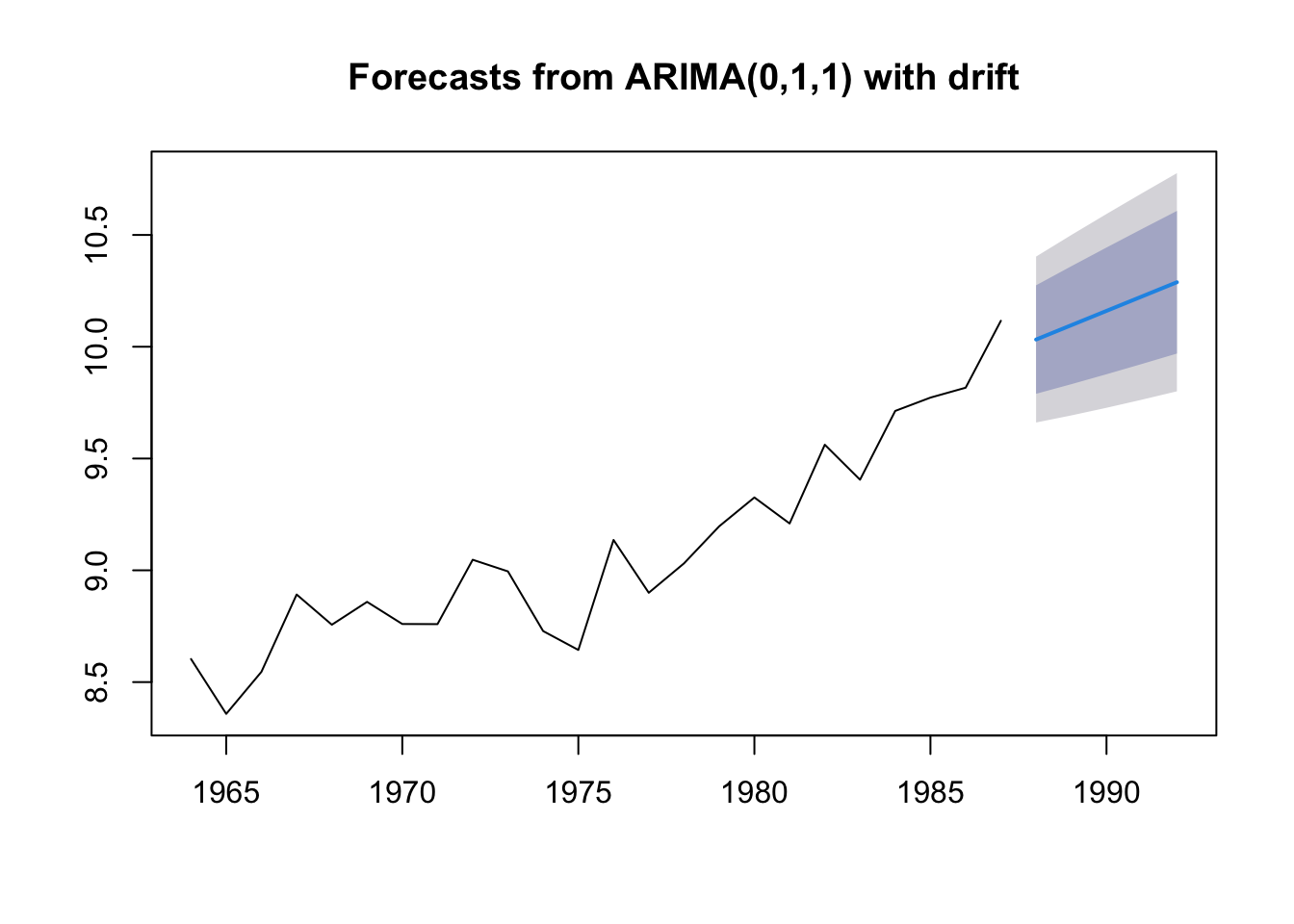
Forecasts for chub mackerel
We can repeat for other species.
spp="Chub.mackerel"
dat <- subset(greeklandings, Species==spp & Year<=1987)$log.metric.tons
dat <- ts(dat, start=1964)
fit <- forecast::auto.arima(dat)
fr <- forecast::forecast(fit, h=5)
plot(fr, ylim=c(6,10))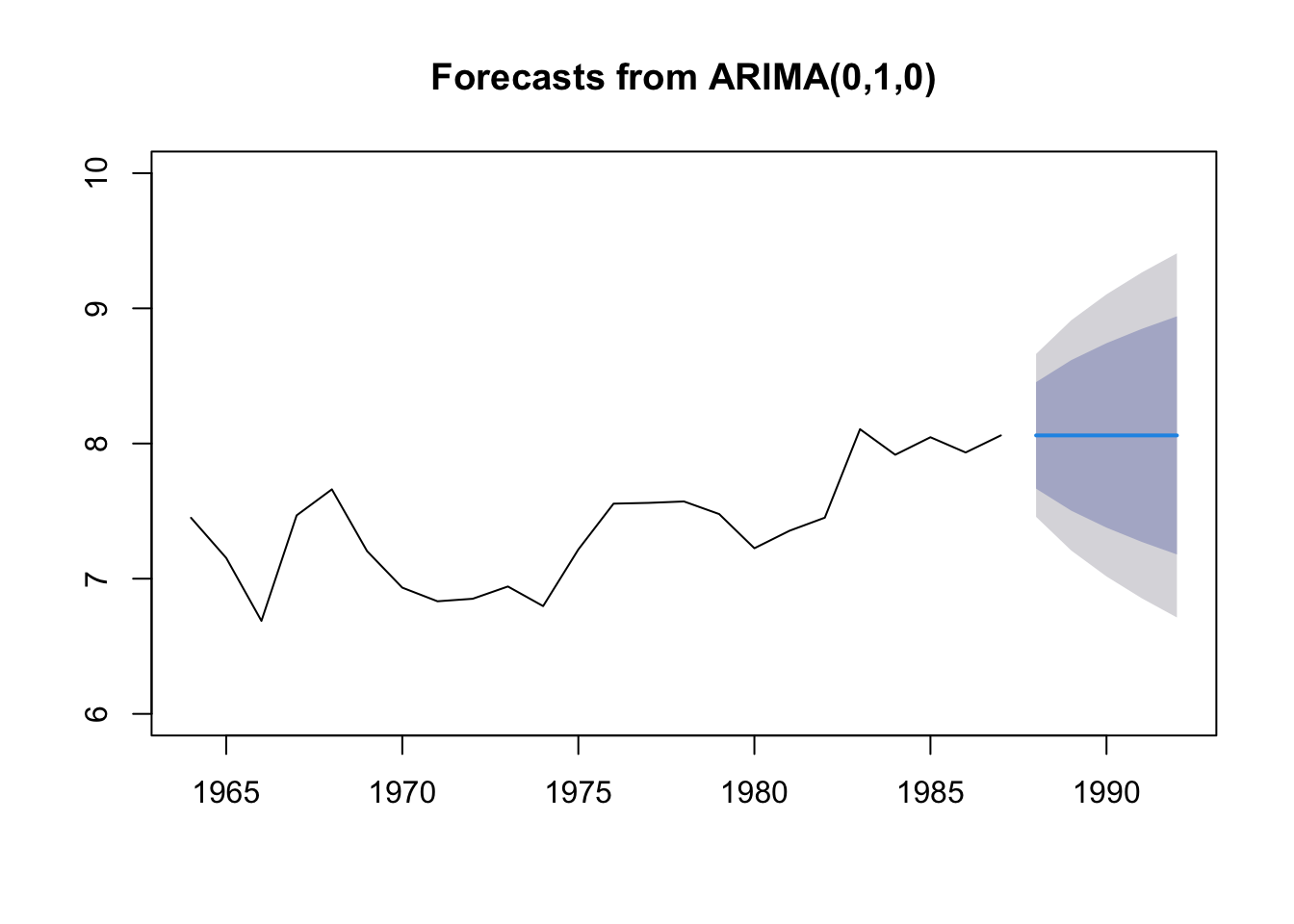
3.5.2 Missing values
Missing values are allowed for arima() and we can product forecasts with the same code.
anchovy.miss <- anchovy87ts
anchovy.miss[10:14] <- NA
fit <- forecast::auto.arima(anchovy.miss)
fr <- forecast::forecast(fit, h=5)
plot(fr)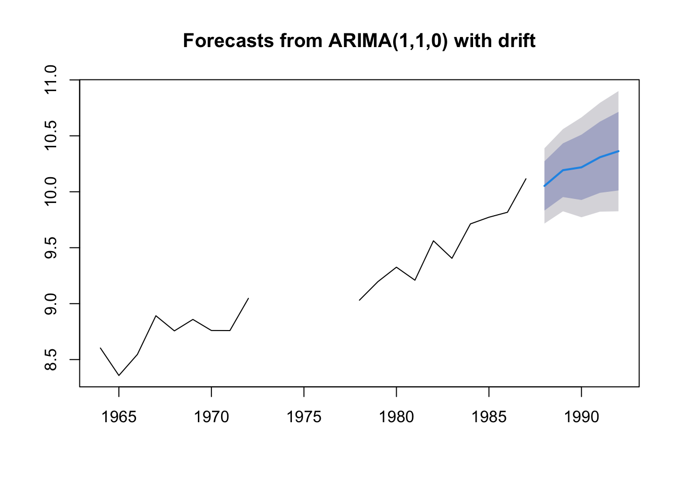
3.5.3 Null forecast models
Whenever we are testing a forecast model or procedure we have developed, we should test against ‘null’ forecast models. These are standard ‘competing’ forecast models.
- The Naive forecast
- The Naive forecast with drift
- The mean or average forecast
The “Naive” forecast
The “naive” forecast is simply the last value observed. If we want to prediction landings in 2019, the naive forecast would be the landings in 2018. This is a difficult forecast to beat! It has the advantage of having no parameters.
In forecast, we can fit this model with the naive() function. Note this is the same as the rwf() function.
fit.naive <- forecast::naive(anchovy87ts)
fr.naive <- forecast::forecast(fit.naive, h=5)
plot(fr.naive)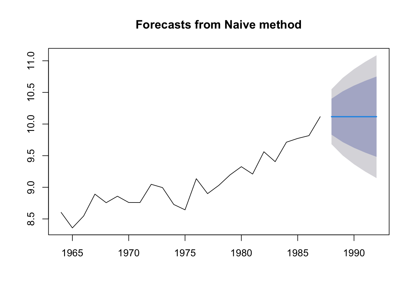
The “Naive” forecast with drift
The “naive” forecast is equivalent to a random walk with no drift. So this \[x_t = x_{t-1} + e_t\] As you saw with the anchovy fit, it doesn’t allow an upward trend. Let’s make it a little more flexible by add drift. This means we estimate one term, the trend.
\[x_t = \mu + x_{t-1} + e_t\]
fit.rwf <- forecast::rwf(anchovy87ts, drift=TRUE)
fr.rwf <- forecast::forecast(fit.rwf, h=5)
plot(fr.rwf)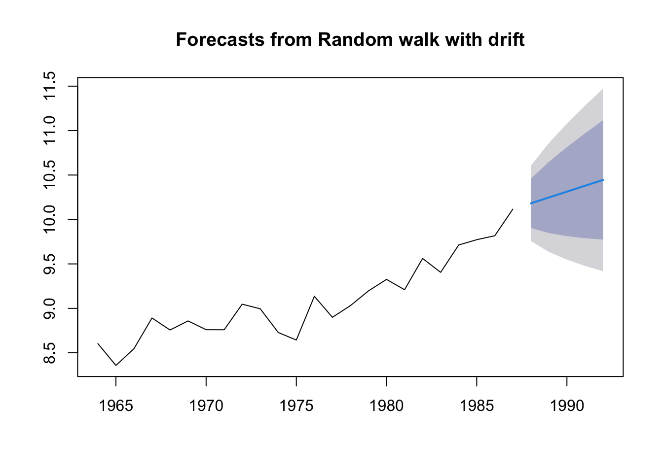
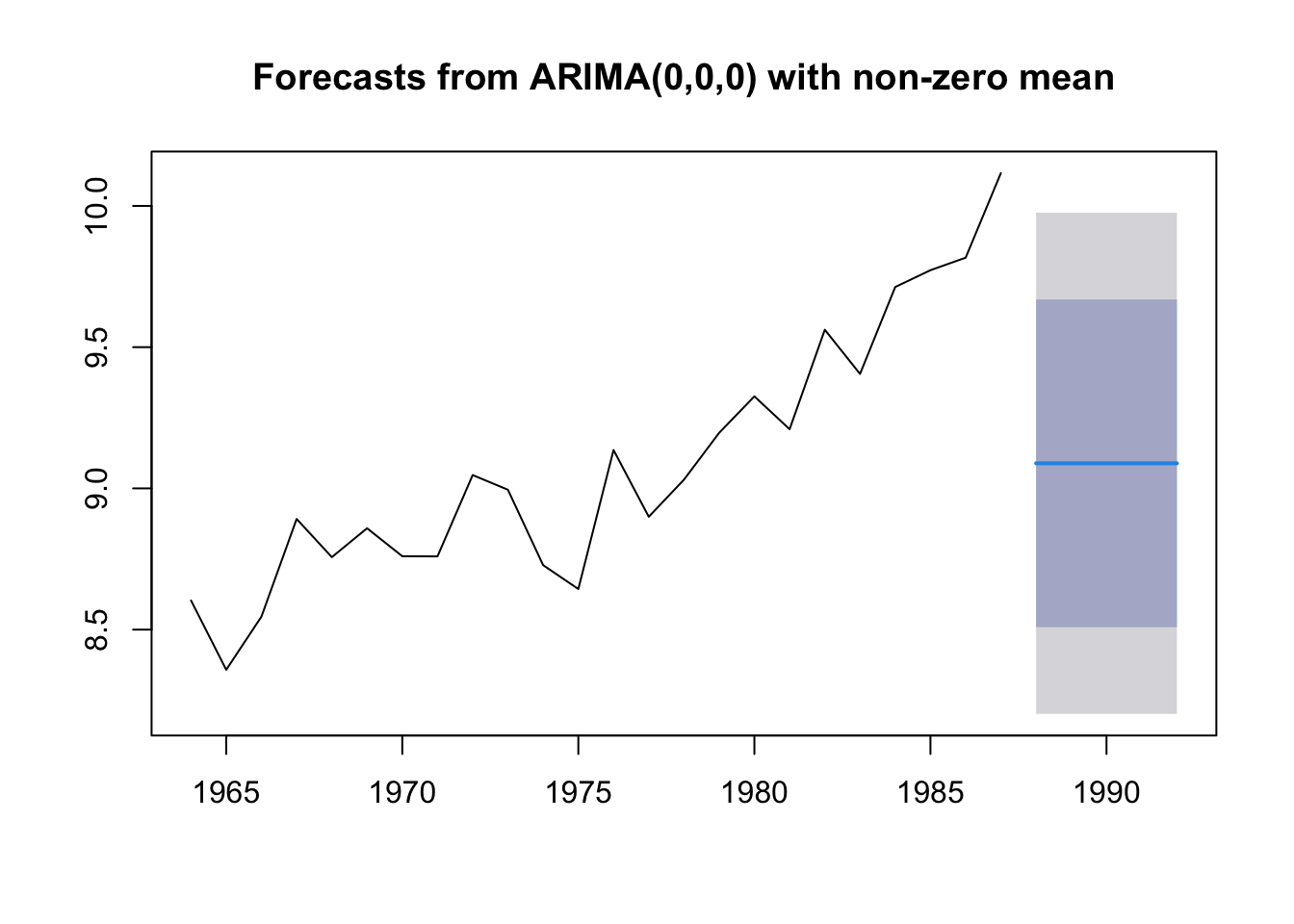
The “mean” forecast
The “mean” forecast is simply the mean of the data. If we want to prediction landings in 2019, the mean forecast would be the average of all our data. This is a poor forecast typically. It uses no information about the most recent values.
In forecast, we can fit this model with the Arima() function and order=c(0,0,0). This will fit this model: \[x_t = e_t\] where \(e_t \sim N(\mu, \sigma)\).
fit.mean <- forecast::Arima(anchovy87ts, order=c(0,0,0))
fr.mean <- forecast::forecast(fit.mean, h=5)
plot(fr.mean)