Chapter 2 Time-varying regression

Time-varying regression is simply a linear regression where time is the explanatory variable:

$$log(catch) = \alpha + \beta t + \beta_2 t^2 + \dots + e_t$$ The error term ( $e_t$ ) was treated as an independent Normal error ( $\sim N(0, \sigma)$ ) in Stergiou and Christou (1996). If that is not a reasonable assumption, then it is simple to fit a non-Gausian error model in R.

Order of the time polynomial

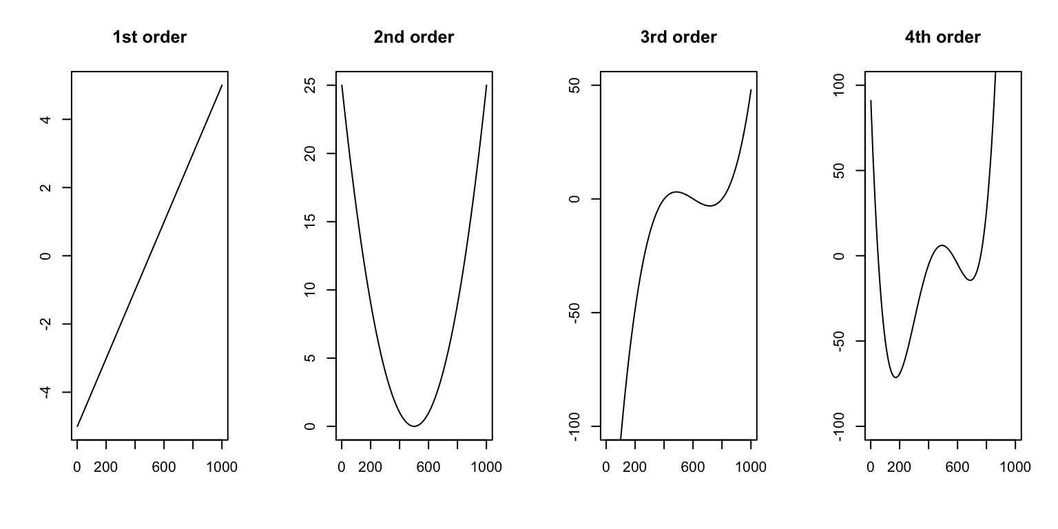
The order of the polynomial of $t$ determines how the time axis (x-axis) relates to the overall trend in the data. A 1st order polynomial ($\beta t$) will allow a linear relationship only. A 2nd order polynomial($\beta_1 t + \beta_2 t^2$) will allow a convex or concave relationship with one peak. 3rd and 4th orders will allow more flexible relationships with more peaks.