6.2 Collinearity

Collinearity is near-linear relationships among the explanatory variables. Collinearity causes many problems such as inflated standard errors of the coefficients and correspondingly unbiased but highly imprecise estimates of the coefficients, false p-values, and poor predictive accuracy of the model. Thus it is important to evaluate the level of collinearity in your explanatory variables.

library(ggplot2)
library(car)
library(Hmisc)
library(corrplot)
library(olsrr)

Pairs plot

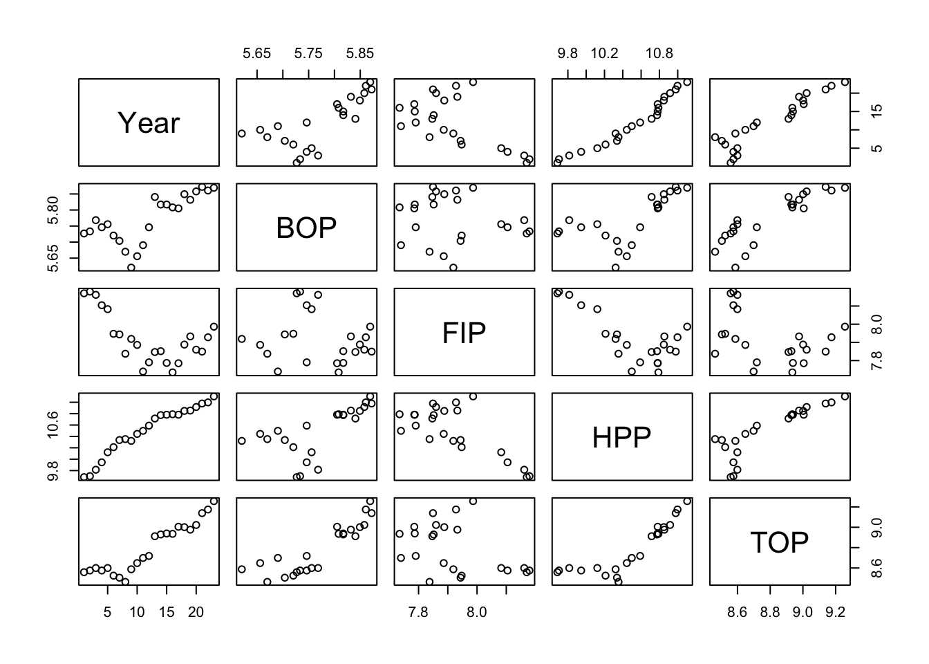
One way to see this is visually is with the pairs() plot. A pairs plot of fishing effort covariates reveals high correlations between Year, HPP and TOP.

pairs(df[,c(2,9:12)])

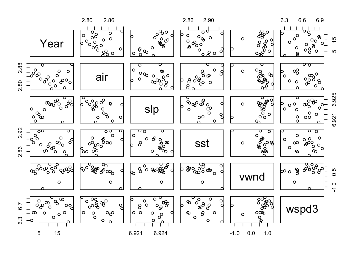
The environmental covariates look generally ok.

pairs(df[,c(2,4:8)])

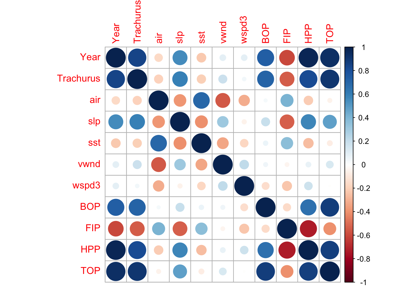
Another way that we can visualize the problem is by looking at the correlation matrix using the corrplot package.

library(corrplot)
X <- as.matrix(df[,colnames(df)!="anchovy"])
corrplot::corrplot(cor(X))

Variance inflation factors

Another way is to look for collinearity is to compute the variance inflation factors (VIF). The variance inflation factor is an estimate of how much larger the variance of a coefficient estimate is compared to if the variable were uncorrelated with the other explanatory variables in the model. If the VIF of variable \(i\) is \(z\), then the standard error of the \(\beta_i\) for variable \(i\) is \(\sqrt{z}\) times larger than if variable \(i\) were uncorrelated with the other variables. For example, if VIF=10, the standard error of the coefficient estimate is 3.16 times larger (inflated). The rule of thumb is that any of the variables with VIF greater than 10 have collinearity problems.

The vif() function in the car package will compute VIFs for us.

full <- lm(anchovy ~ ., data=df)
car::vif(full)

##       Year  Trachurus        air        slp        sst       vwnd      wspd3 
## 103.922970  18.140279   3.733963   3.324463   2.476689   2.010485   1.909992 
##        BOP        FIP        HPP        TOP 
##  13.676208   8.836446  63.507170 125.295727

The ols_vif_tol() function in the olsrr package also computes the VIF.

olsrr::ols_vif_tol(full)

(#tab:vif.olsrr)
Variables	Tolerance	VIF
Year	0.00962	104
Trachurus	0.0551	18.1
air	0.268	3.73
slp	0.301	3.32
sst	0.404	2.48
vwnd	0.497	2.01
wspd3	0.524	1.91
BOP	0.0731	13.7
FIP	0.113	8.84
HPP	0.0157	63.5
TOP	0.00798	125

This shows that Year, HPP and TOP have severe collinearity problems, and BOP and Trachusus also have collinearity issues, though lesser.

Condition indices

Condition indices are computed from the eigenvalues of the correlation matrix of the variates. The size of the index will be greatly affected by whether you have standardized the variance of your covariates, unlike the other tests described here.

\[ci = \sqrt{max(eigenvalue)/eigenvalue}\]

vars <- as.matrix(dfz[,-1])
res <- eigen(crossprod(vars))$values
sqrt(max(res)/res)

##  [1]  1.000000  1.506975  2.235652  2.332424  3.025852  3.895303  4.753285
##  [8]  5.419310  7.977486 20.115739 35.515852

vars <- as.matrix(dfz[,-1])
res <- eigen(crossprod(vars))$values
sqrt(max(res)/res)

##  [1]  1.000000  1.506975  2.235652  2.332424  3.025852  3.895303  4.753285
##  [8]  5.419310  7.977486 20.115739 35.515852

See the information from the olsrr package on condition indices on how to use condition indices to spot collinearity. Basically you are looking for condition indices greater than 30 whether the proportion of variance for the covariate is greater than 0.5. In the table below, this criteria identifies Year, BOP, and TOP. Note that the test was done with the standardized covariates (dfz).

model <- lm(anchovy ~ ., data=dfz)
round(olsrr::ols_eigen_cindex(model), digit=2)

Table 6.1:
Eigenvalue	Condition Index	intercept	Year	Trachurus	air	slp	sst	vwnd	wspd3	BOP	FIP	HPP	TOP
5.25	1	0	0	0	0	0.01	0	0	0	0	0	0	0
2.31	1.51	0	0	0	0.03	0	0.04	0.03	0.02	0	0	0	0
1.05	2.24	0	0	0	0	0.01	0	0.13	0.17	0	0.02	0	0
1	2.29	1	0	0	0	0	0	0	0	0	0	0	0
0.96	2.33	0	0	0	0	0.05	0.02	0.1	0.21	0.01	0.01	0	0
0.57	3.03	0	0	0	0.03	0.15	0.24	0.12	0.01	0.02	0	0	0
0.35	3.9	0	0	0	0.14	0.13	0.24	0.04	0.16	0.01	0.09	0	0
0.23	4.75	0	0	0.02	0.33	0.15	0.15	0.45	0.07	0.01	0.03	0	0
0.18	5.42	0	0.01	0.18	0.09	0.09	0.08	0.01	0	0	0.03	0.01	0
0.08	7.98	0	0.02	0.04	0.23	0.29	0.09	0.01	0.16	0.4	0.12	0	0
0.01	20.1	0	0.05	0.29	0.02	0.04	0.07	0.04	0.13	0	0.67	0.64	0.15
0	35.5	0	0.92	0.47	0.12	0.09	0.06	0.07	0.06	0.55	0.01	0.35	0.84

redun()

The Hmisc library also has a redundancy function (redun()) that can help identify which variables are redundant. This identifies variables that can be explained with an \(R^2>0.9\) by a linear (or non-linear) combination of other variables. We are fitting a linear model, so we set nk=0 to force redun() to only look at linear combinations.

We use redun() only on the explanatory variables and thus remove the first column, which is our response variable (anchovy).

a <- Hmisc::redun(~ .,data=df[,-1], nk=0)
a$Out

## [1] "TOP" "HPP"

This indicates that TOP and HPP can be explained by the other variables.

6.2.1 Effect of collinearity

One thing that happens when we have collinearity is that we will get “complementary” (negative matched by positive) and very large coefficients in the variables that are collinear. We see this when we fit a linear regression with all the variables. I use the z-scored data so that the effect sizes (x-axis) are on the same scale.

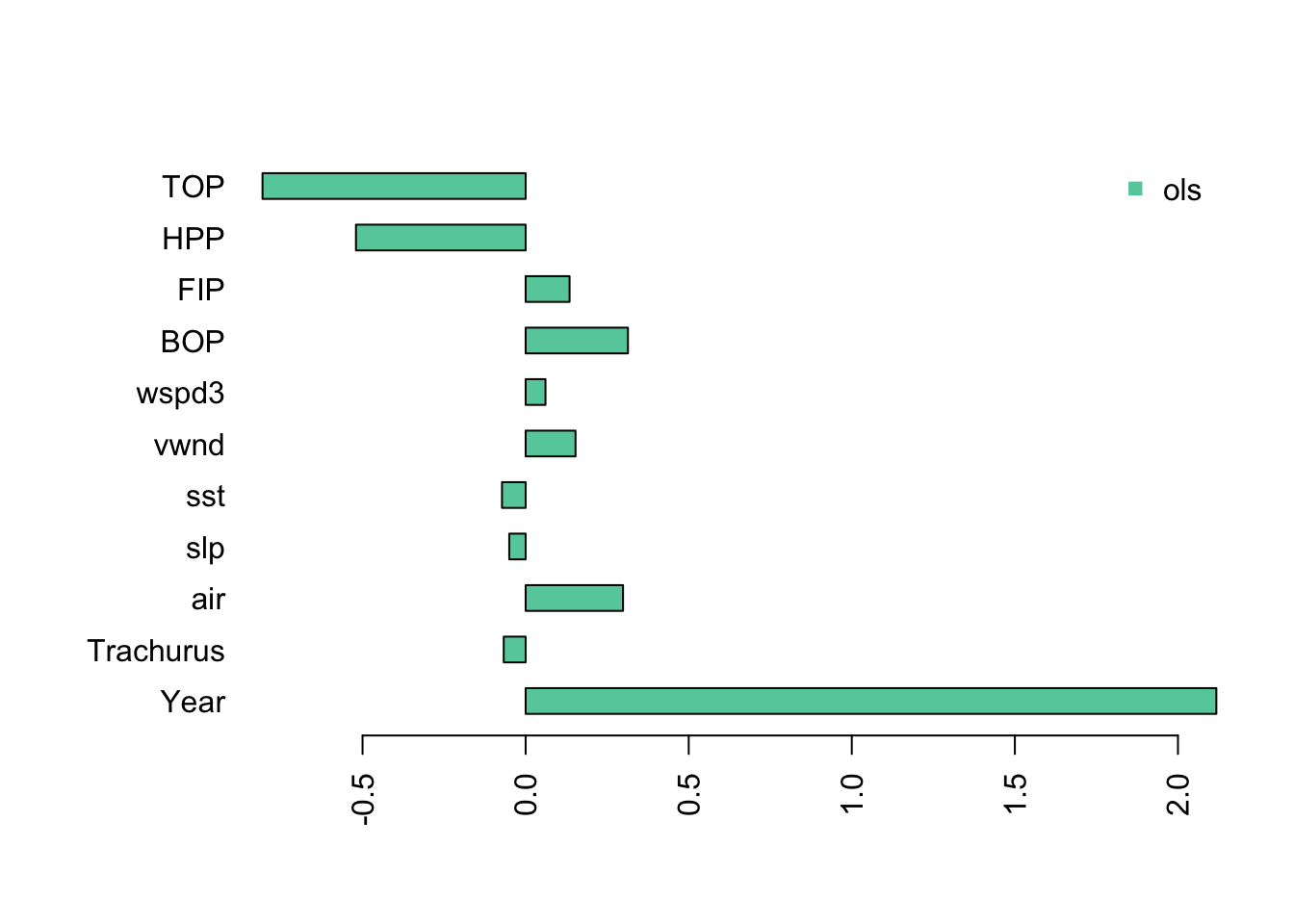
The Year coefficients is very large and the TOP and HPP coefficients are negative and very large. If we look at the fit, we see the at the standard errors for Year, TOP and HPP are very large. The p-value for Year is significant, however in the presence of severe collinearity, reported p-values should not be trusted.

summary(fit.full)

## 
## Call:
## lm(formula = anchovy ~ ., data = dfz)
## 
## Residuals:
##     Min      1Q  Median      3Q     Max 
## -0.4112 -0.1633 -0.0441  0.1459  0.5009 
## 
## Coefficients:
##               Estimate Std. Error t value Pr(>|t|)  
## (Intercept) -9.175e-15  7.003e-02   0.000   1.0000  
## Year         2.118e+00  7.139e-01   2.966   0.0128 *
## Trachurus   -6.717e-02  2.983e-01  -0.225   0.8260  
## air          2.987e-01  1.353e-01   2.207   0.0495 *
## slp         -5.023e-02  1.277e-01  -0.393   0.7016  
## sst         -7.250e-02  1.102e-01  -0.658   0.5242  
## vwnd         1.530e-01  9.930e-02   1.540   0.1517  
## wspd3        6.086e-02  9.679e-02   0.629   0.5423  
## BOP          3.137e-01  2.590e-01   1.211   0.2512  
## FIP          1.347e-01  2.082e-01   0.647   0.5309  
## HPP         -5.202e-01  5.581e-01  -0.932   0.3713  
## TOP         -8.068e-01  7.839e-01  -1.029   0.3255  
## ---
## Signif. codes:  0 '***' 0.001 '**' 0.01 '*' 0.05 '.' 0.1 ' ' 1
## 
## Residual standard error: 0.3359 on 11 degrees of freedom
## Multiple R-squared:  0.946,	Adjusted R-squared:  0.8921 
## F-statistic: 17.53 on 11 and 11 DF,  p-value: 2.073e-05

Stergiou and Christou do not state how (if at all) they address the collinearity in the explanatory variables, but it is clearly present. In the next chapter, I will show how to develop a multivariate regression model using variable selection. This is the approach used by Stergiou and Christou. Keep in mind that variable selection will not perform well when there is collinearity in your covariates and that variable selection is prone to over-fitting and selecting covariates due to chance.