4.2 ets() function

The ets() function in the forecast package fits exponential smoothing models and produces forecasts from the fitted models. It also includes functions for plotting forecasts.

Load the data by loading the FishForecast package.

require(FishForecast)

Fit the model.

fit <- forecast::ets(anchovy87ts, model="ANN")

model="ANN" specifies the simple exponential smoothing model.

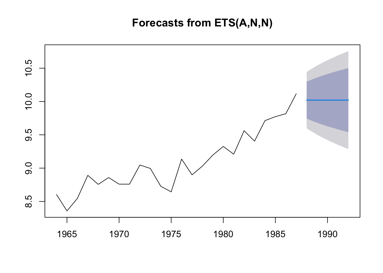
Create a forecast for 5 time steps into the future.

fr <- forecast::forecast(fit, h=5)

Plot the forecast.

plot(fr)

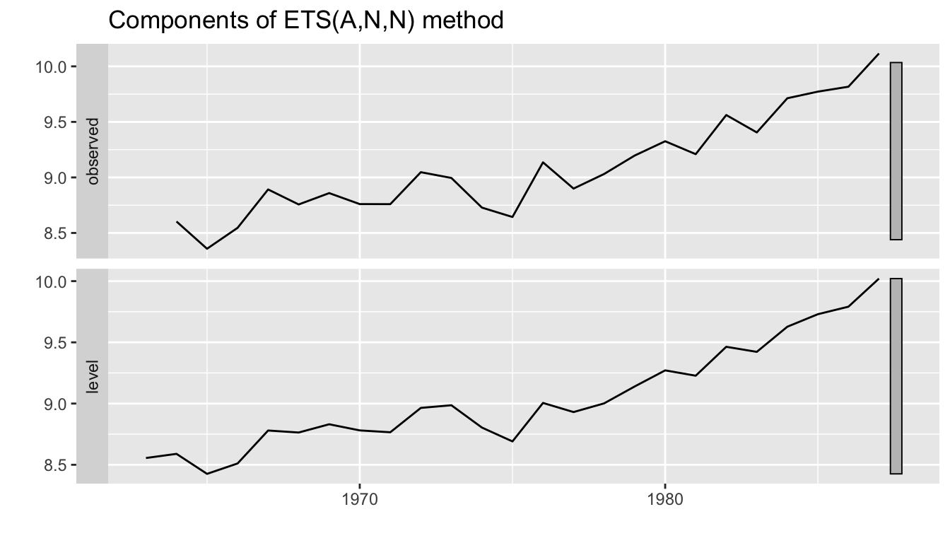
Look at the estimates

fit

## ETS(A,N,N) 
## 
## Call:
##  forecast::ets(y = anchovy87ts, model = "ANN") 
## 
##   Smoothing parameters:
##     alpha = 0.7065 
## 
##   Initial states:
##     l = 8.5553 
## 
##   sigma:  0.2166
## 
##       AIC      AICc       BIC 
##  6.764613  7.964613 10.298775

4.2.1 The weighting function

The first coefficient of the ets fit is the $\alpha$ parameter for the weighting function.

alpha <- coef(fit)[1]
wts <- alpha*(1-alpha)^(0:23)
plot(1987:1964, wts/sum(wts), lwd=2, ylab="weight", xlab="", type="l")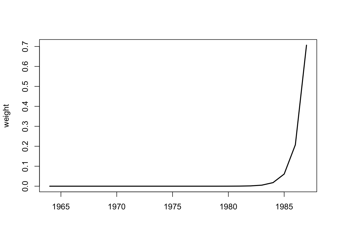

(#fig:ann.weighting)Weighting function for the simple exponential smoothing model for anchovy.

4.2.2 Decomposing your model fit

Sometimes you would like to see the smoothed level that the model estimated. You can see that with plot(fit) or autoplot(fit).

autoplot(fit)

Figure 4.1: Decompositon of an ets fit.