8.1 Chinook data
We will illustrate the analysis of seasonal catch data using a data set of monthly chinook salmon from Washington state.
Load the chinook salmon data set
This is in the FishForecast package.
| Year | Month | Species | State | log.metric.tons | metric.tons | Value |
|---|---|---|---|---|---|---|
| 1990 | Jan | Chinook | WA | 3.4 | 29.9 | 1.09e+05 |
| 1990 | Feb | Chinook | WA | 3.81 | 45.1 | 3.09e+05 |
| 1990 | Mar | Chinook | WA | 3.51 | 33.5 | 2.01e+05 |
| 1990 | Apr | Chinook | WA | 4.25 | 70 | 4.31e+05 |
| 1990 | May | Chinook | WA | 5.2 | 181 | 8.6e+05 |
| 1990 | Jun | Chinook | WA | 4.37 | 79.2 | 4.2e+05 |
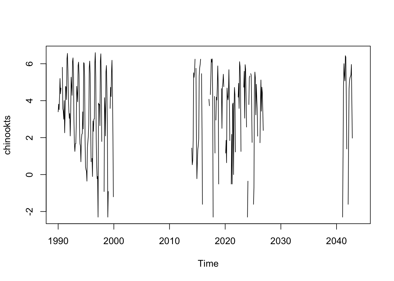
The data are monthly and start in January 1990. To make this into a ts object do
start is the year and month and frequency is the number of months in the year. If we had quarterly data that started in 2nd quarter of 1990, our call would be
ts(chinook$log.metric.tons, start=c(1990,2), frequency=4)If we had daily data starting on hour 5 of day 10 and each row was an hour, our call would be
ts(chinook$log.metric.tons, start=c(10,5), frequency=24)Use ?ts to see more examples of how to set up ts objects.