6.4 Penalized regression

The problem with model selection using searching and selecting with some model fit criteria is that the selected model tends to be over-fit—even when using cross-validation. The predictive value of the model is not optimal because of over-fitting. Another approach to dealing with variance inflation that arises from collinearity and models with many explanatory variable is penalized regression. The basic idea with penalized regression is that you penalize coefficient estimates that are far from 0. The true coefficients are (likely) not 0 so fundamentally this will lead to biased coefficient estimates but the idea is that the inflated variance of the coefficient estimates is the bigger problem.

6.4.1 Ridge Regression

First, let’s look at ridge regression. With ridge regression, we will assume that the coefficients have a mean of 0 and a variance of \(1/\lambda\). This is our prior on the coefficients. The \(\beta_i\) are the most probable values given the data and the prior. Note, there are many other ways to derive ridge regression.

We will use the glmnet package to fit the anchovy catch with ridge regression. To fit with a ridge penalty, we set alpha=0.

library(glmnet)
resp <- colnames(dfz)!="anchovy"
x <- as.matrix(dfz[,resp])
y <- as.matrix(dfz[,"anchovy"])
fit.ridge <- glmnet(x, y, family="gaussian", alpha=0)

We need to choose a value for the penalty parameter \(\lambda\) (called s in coef.glmnet()). If \(\lambda\) is large, then our prior is that the coefficients are very close to 0. If our \(\lambda\) is small, then our prior is less informative.

We can use cross-validation to choose \(\lambda\). This chooses a \(\lambda\) that gives us the lowest out of sample errors. cv.glmnet() will do k-fold cross-validation and report the MSE. We pick the \(\lambda\) with the lowest MSE (lambda.min) or the largest value of \(\lambda\) such that error is within 1 s.e. of the minimum (lambda.1se). This value is computed via cross-validation so will vary. We will take the average over a number of runs; here 20 for speed but 100 is better.

Once we have a best \(\lambda\) to use, we can get the coefficients at that value.

n <- 20; s <- 0
for(i in 1:n) s <- s + cv.glmnet(x, y, nfolds=5, alpha=0)$lambda.min
s.best.ridge <- s/n
coef(fit.ridge, s=s.best.ridge)

## 12 x 1 sparse Matrix of class "dgCMatrix"
##                         1
## (Intercept) -1.025097e-14
## Year         5.417884e-01
## Trachurus   -1.828772e-01
## air          1.897000e-01
## slp         -8.056669e-02
## sst         -8.958912e-02
## vwnd         8.140451e-02
## wspd3        2.616673e-02
## BOP          9.399500e-02
## FIP          1.156512e-01
## HPP          3.036030e-01
## TOP          2.358358e-01

I will plot the standardized coefficients for the ordinary least squares coefficients against the coefficients using ridge regression.

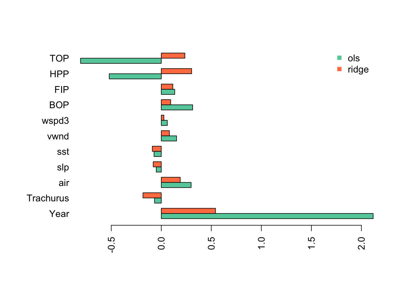
This shows the problem caused by the highly collinear TOP and HPP. They have highly inflated coefficient estimates that are offset by an inflated Year coefficient (in the opposite direction). This is why we need to evaluate collinearity in our variables before fitting a linear regression.

With ridge regression, all the estimates have shrunk towards 0 (as they should) but the collinear variables still have very large coefficients.

6.4.2 Lasso

In ridge regression, the coefficients will be shrunk towards 0 but none will be set to 0 (unless the OLS estimate happens to be 0). Lasso is a type of regression that uses a penalty function where 0 is an option. Lasso does a combination of variable selection and shrinkage.

We can do lasso with glmnet() by setting alpha=1.

fit.lasso <- glmnet(x, y, family="gaussian", alpha=1)

We select the best \(\lambda\) as we did for ridge regression using cross-validation.

n <- 20; s <- 0
for(i in 1:n) s <- s + cv.glmnet(x, y, nfolds=5, alpha=1)$lambda.min
s.best.lasso <- s/n
coef.lasso <- as.vector(coef(fit.lasso, s=s.best.lasso))[-1]

We can compare to the estimates from ridge and OLS and see that the model is now more similar the models we got from stepwise variable selection. The main difference is that slp and air are included as variables.

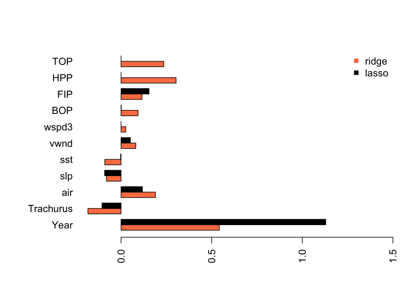
Lasso has estimated a model that is similar to what we got with stepwise variable selection without removing the collinear variables from our data set.

6.4.3 Elastic net

Elastic net is uses both L1 and L2 regularization. Elastic regression generally works well when we have a big dataset. We do not have a big dataset but we will try elastic net. You can tune the amount of L1 and L2 mixing by adjusting alpha but for this example, we will just use alpha=0.5.

fit.en <- glmnet(x, y, family="gaussian", alpha=0.5)
n <- 20; s <- 0
for(i in 1:n) s <- s + cv.glmnet(x, y, nfolds=5, alpha=0.5)$lambda.min
s.best.el <- s/n
coef.en <- as.vector(coef(fit.en, s=s.best.el))[-1]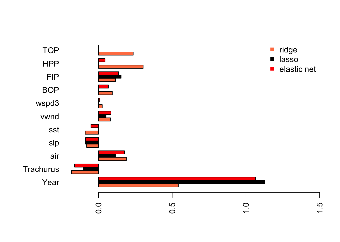

As we might expect, elastic net is part way between the ridge regression model and the Lasso model.