3.1 Overview
3.1.1 Components of an ARIMA model
You will commonly see ARIMA models referred to as Box-Jenkins models. This model has 3 components (p, d, q):
- AR autoregressive \(y_t\) depends on past values. The AR level is maximum lag \(p\).
\[x_t = \phi_1 x_{t-1} + \phi_2 x_{t-2} + ... + \phi_p x_{t-p} + e_t\]
- I differencing \(x_t\) may be a difference of the observed time series. The number of differences is denoted \(d\). First difference is \(d=1\):
\[x_t = y_t - y_{t-1}\]
- MA moving average The error \(e_t\) can be a sum of a time series of independent random errors. The maximum lag is denoted \(q\).
\[e_t = \eta_t + \theta_1 \eta_{t-1} + \theta_2 \eta_{t-2} + ... + \theta_q \eta_{t-q},\quad \eta_t \sim N(0, \sigma)\]
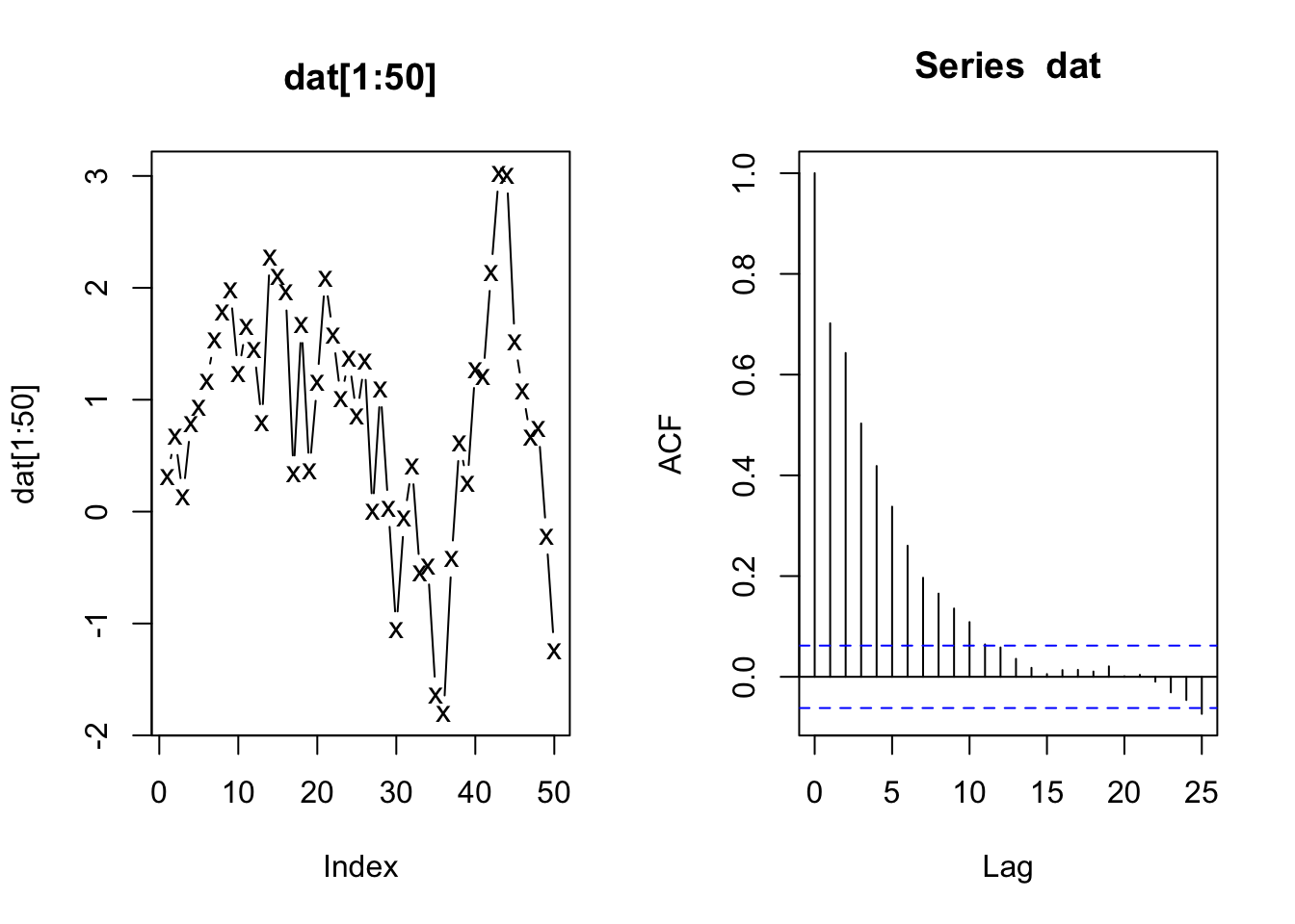
Create some data from an AR(2) Model
\[x_t = 0.5 x_{t-1} + 0.3 x_{t-2} + e_t\]
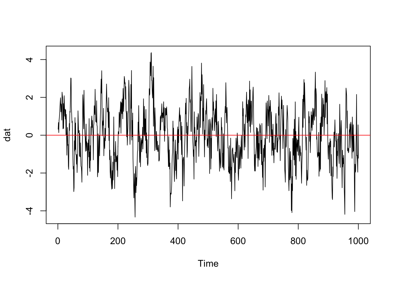
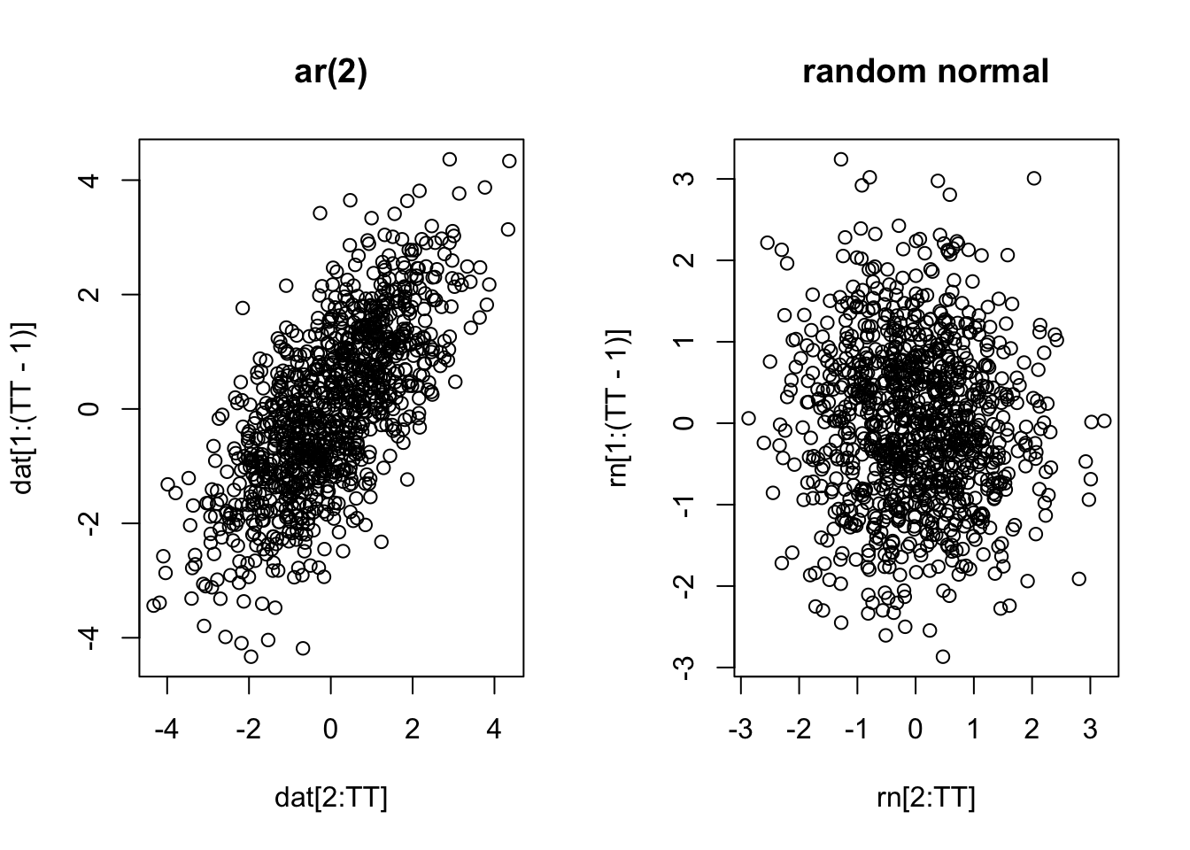
Compare AR(2) and random data.
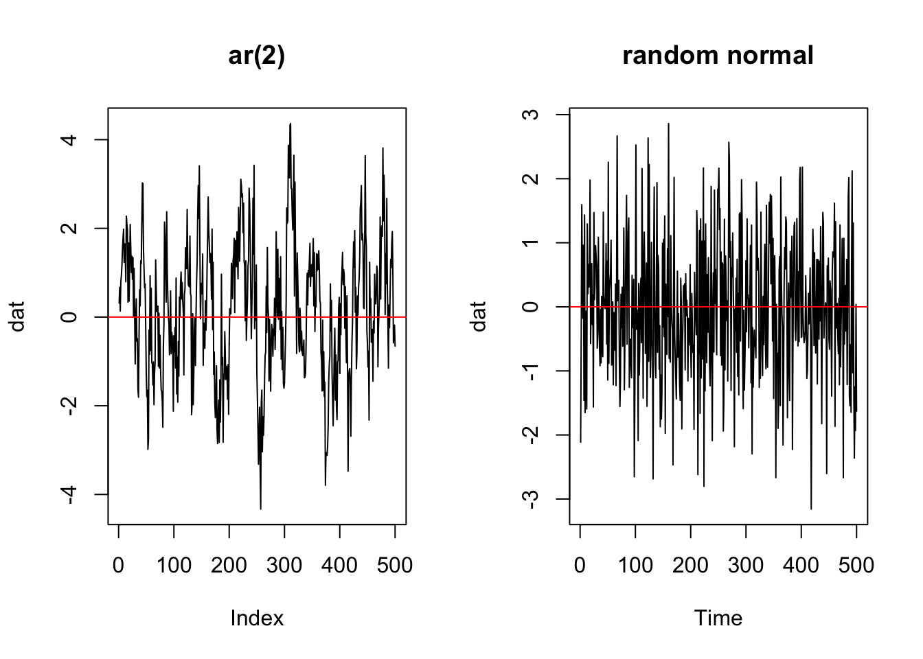
AR(2) is auto-correlated
Plot the data at time \(t\) against the data at time \(t-1\)
3.1.2 Box-Jenkins method
This refers to a step-by-step process of selecting a forecasting model. You need to go through the steps otherwise you could end up fitting a nonsensical model or using fitting a sensible model with an algorithm that will not work on your data.
A. Model form selection
- Evaluate stationarity and seasonality
- Selection of the differencing level (d)
- Selection of the AR level (p)
- Selection of the MA level (q)
B. Parameter estimation
C. Model checking
3.1.3 ACF and PACF functions
The ACF function
The auto-correlation function (ACF) is the correlation between the data at time \(t\) and \(t+1\). This is one of the basic diagnostic plots for time series data.
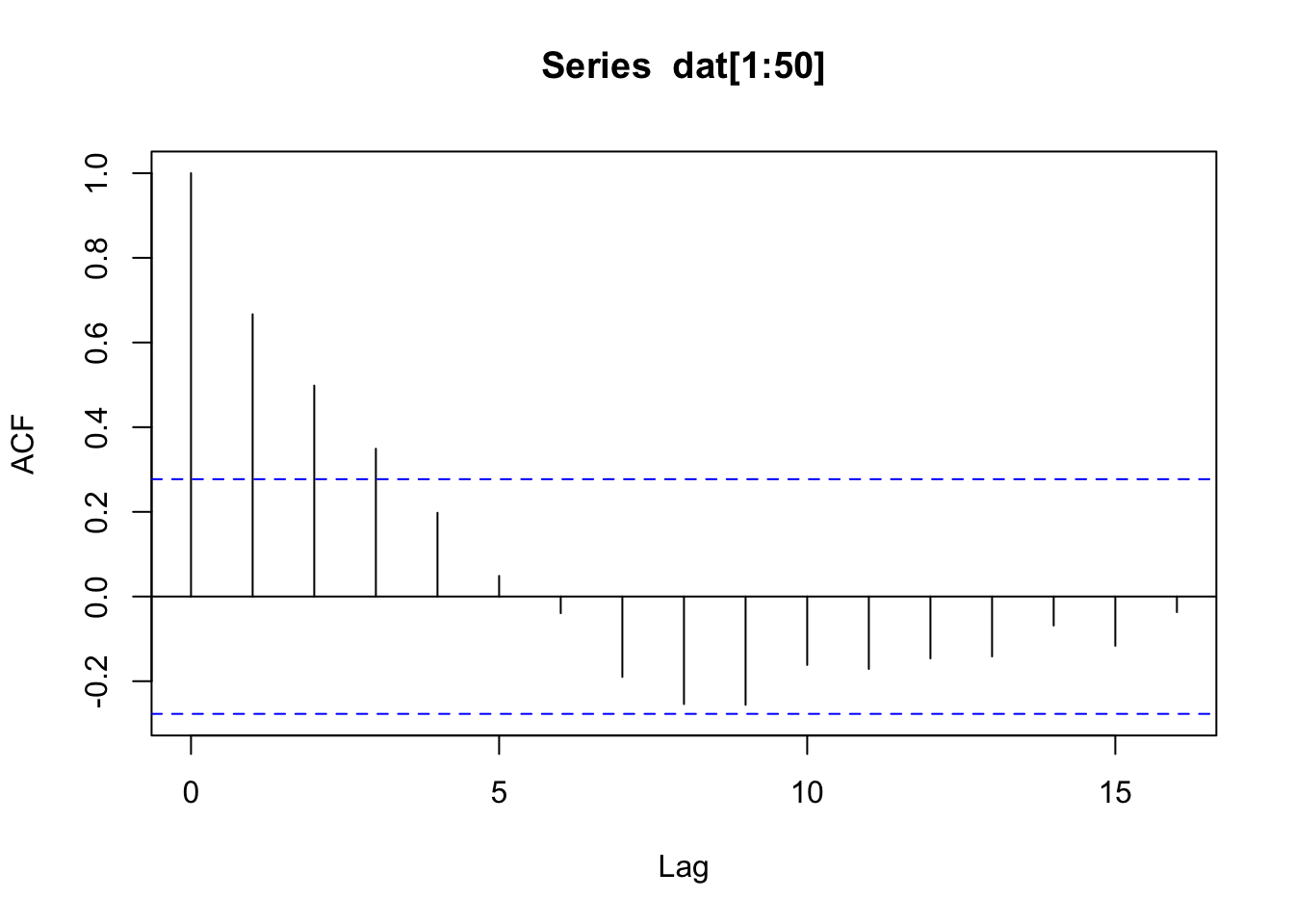
The ACF simply shows the correlation between all the data points that are lag \(p\) apart. Here are the correlations for points lag 1 and lag 10 apart. cor() is the correlation function.
## [1] 0.7022108## [1] 0.1095311The values match what we see in the ACF plot.
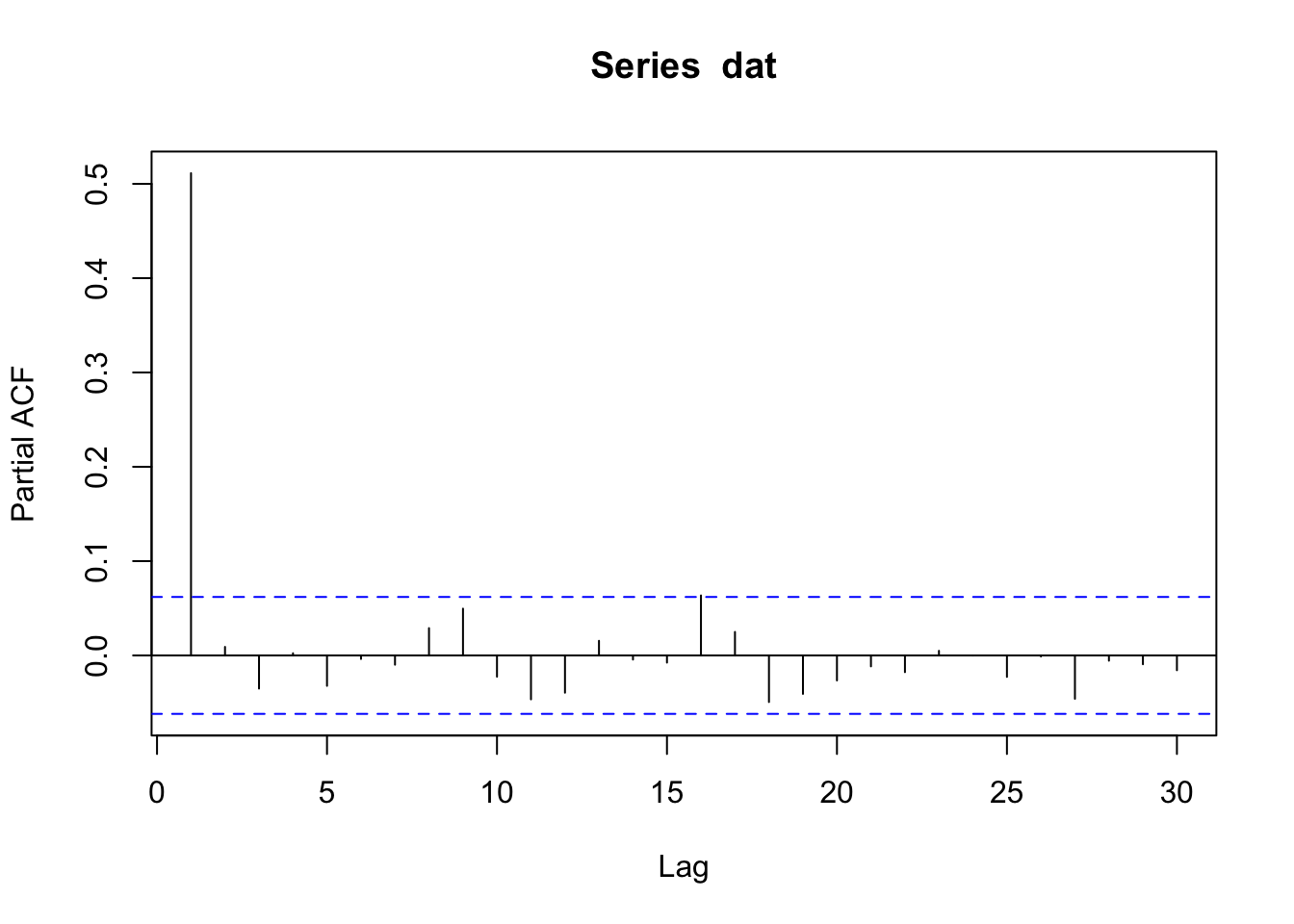
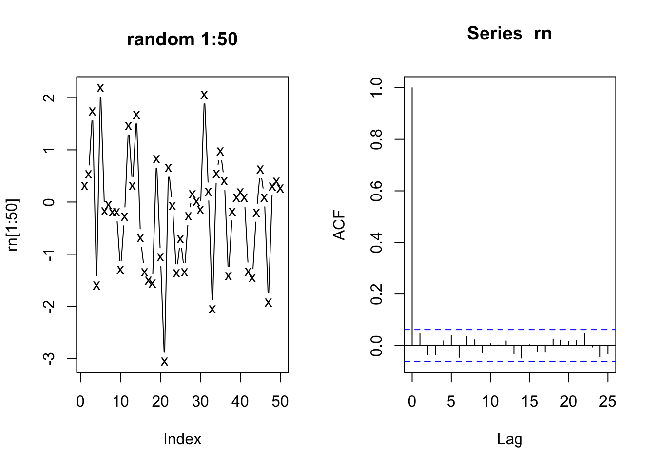
ACF for independent data
Temporally independent data shows no significant autocorrelation.
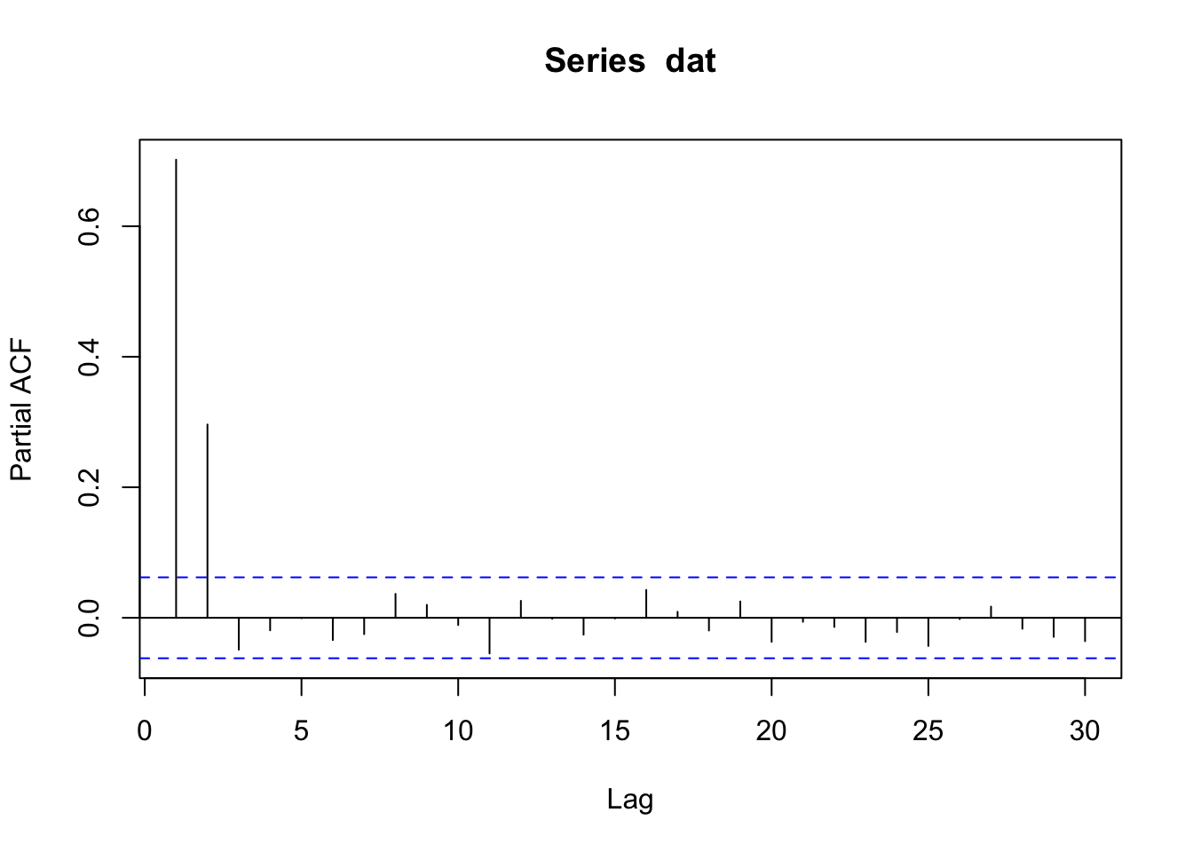
PACF function
In the ACF for the AR(2), we see that \(x_t\) and \(x_{t-3}\) are correlated even those the model for \(x_t\) does not include \(x_{t-3}\). \(x_{t-3}\) is correlated with \(x_t\) indirectly because \(x_{t-3}\) is directly correlated with \(x_{t-2}\) and \(x_{t-1}\) and these two are in turn directly correlated with \(x_t\). The partial autocorrelation function removes this indirect correlation. Thus the only significant lags in the PACF should be the lags that appear in the process model.
For example, if the model is
Partial ACF for AR(2)
\[x_t = 0.5 x_{t-1} + 0.3 x_{t-2} + e_t\] then only the first two lags should be significant in the PACF.