7.1 Seasonal Exponential Smoothing Model
Now we add a few more lines to our ETS table of models:
| model | “ZZZ” | alternate function |
|---|---|---|
| exponential smoothing no trend | “ANN” | ses() |
| exponential smoothing with trend | “AAN” | holt() |
| exponential smoothing with season no trend | “ANA” | NA |
| exponential smoothing with season and trend | “AAA” | NA |
| estimate best trend and season model | “ZZZ” | NA |
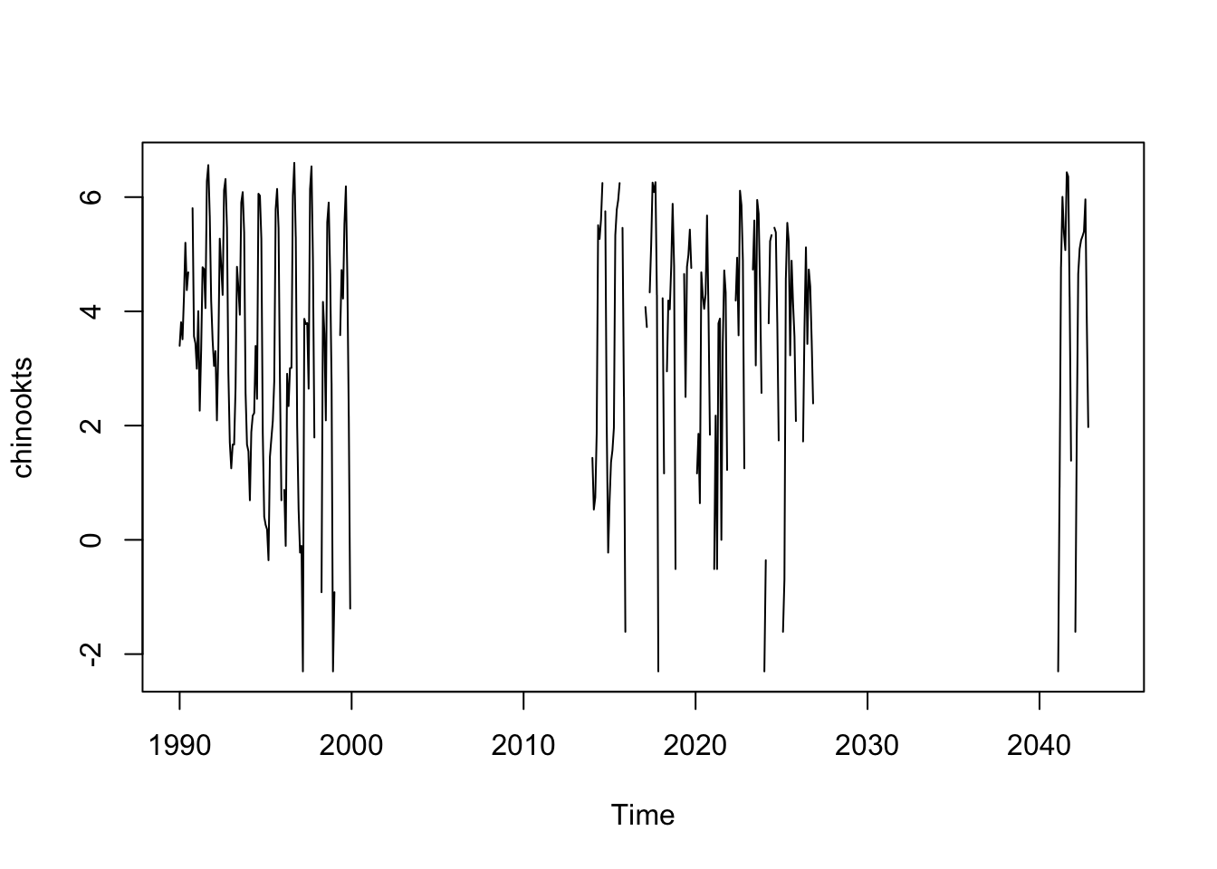
Unfortunately ets() will not handle missing values and will find the longest continuous piece of our data and use that.
library(forecast)
traindat <- window(chinookts, c(1990,1), c(1999,12))
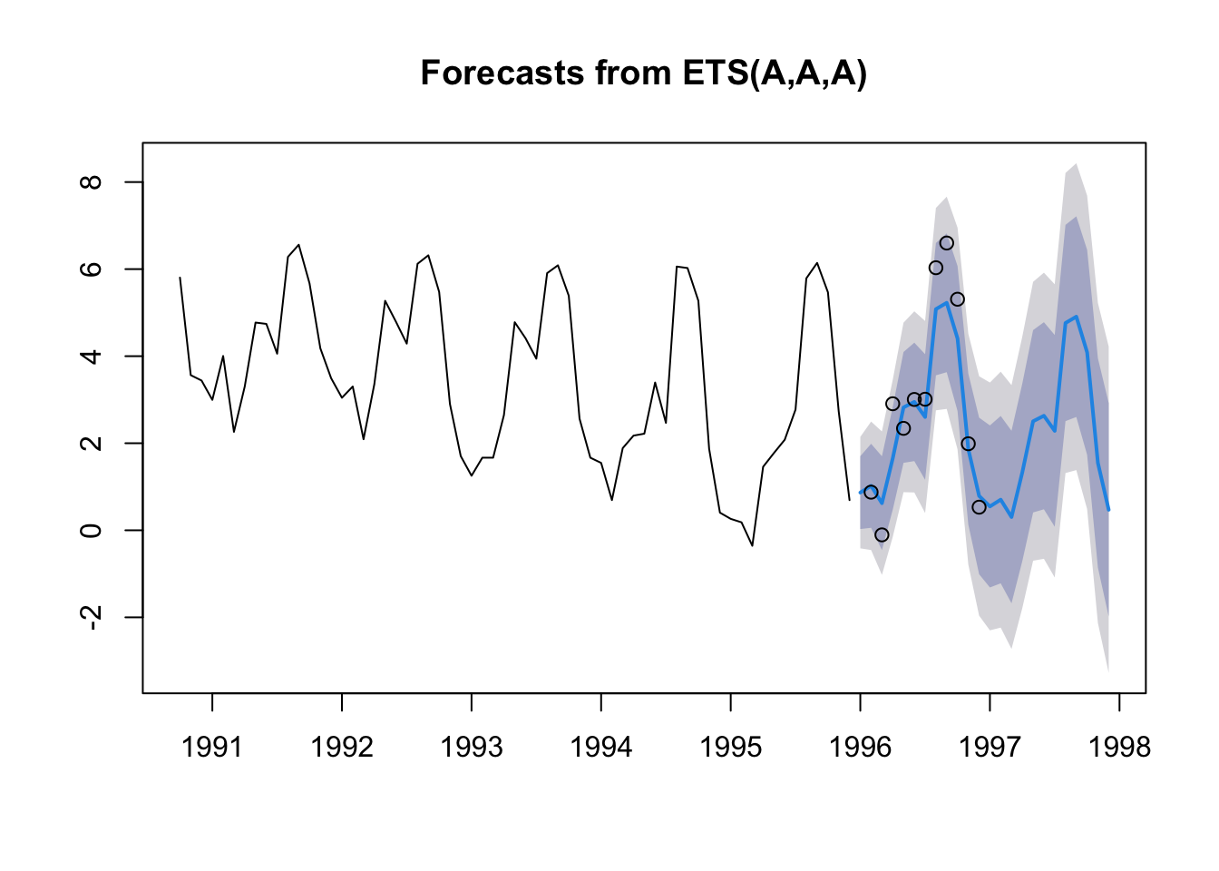
fit <- forecast::ets(traindat, model="AAA")
## Warning in forecast::ets(traindat, model = "AAA"): Missing values
## encountered. Using longest contiguous portion of time seriesfr <- forecast::forecast(fit, h=24)
plot(fr)
points(window(chinookts, c(1996,1), c(1996,12)))
7.1.1 Force seasonality to evolve more
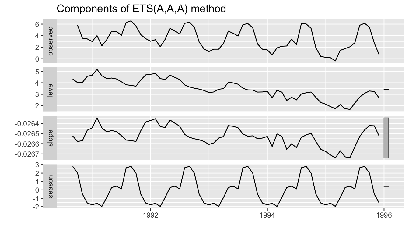
If we plot the decomposition, we see the the seasonal component is not changing over time, unlike the actual data. The bar on the right, alerts us that the scale on the 3rd panel is much smaller.
autoplot(fit)
Pass in a high gamma (the season weighting) to force the seasonality to evolve.
fit <- forecast::ets(traindat, model="AAA", gamma=0.4)## Warning in forecast::ets(traindat, model = "AAA", gamma = 0.4): Missing
## values encountered. Using longest contiguous portion of time seriesautoplot(fit)