2.2 Forecasting with a time-varying regression model
Forecasting is easy in R once you have a fitted model. Let’s say for the anchovy, we fit the model
\[C_t = \alpha + \beta t + e_t\] where \(t\) starts at 1 (so 1964 is \(t=1\) ). To predict, predict the catch in year t, we use
\[C_t = \alpha + \beta t + e_t\]
Model fit:
load("landings.RData")
anchovy87$t <- anchovy87$Year-1963
model <- lm(log.metric.tons ~ t, data=anchovy87)
coef(model)
## (Intercept) t
## 8.36143085 0.05818942For anchovy, the estimated \(\alpha\) (Intercept) is 8.3614309 and \(\beta\) is 0.0581894. We want to use these estimates to forecast 1988 ( \(t=25\) ).
So the 1988 forecast is 8.3614309 + 0.0581894 \(\times\) 25 :
coef(model)[1]+coef(model)[2]*25## (Intercept)
## 9.816166log metric tons.
2.2.1 The forecast package
The forecast package in R makes it easy to create forecasts with fitted models and to plot (some of) those forecasts.
For a TV Regression model, our forecast() call looks like
fr <- forecast::forecast(model, newdata = data.frame(t=25:29))The dark grey bands are the 80% prediction intervals and the light grey are the 95% prediction intervals.
plot(fr)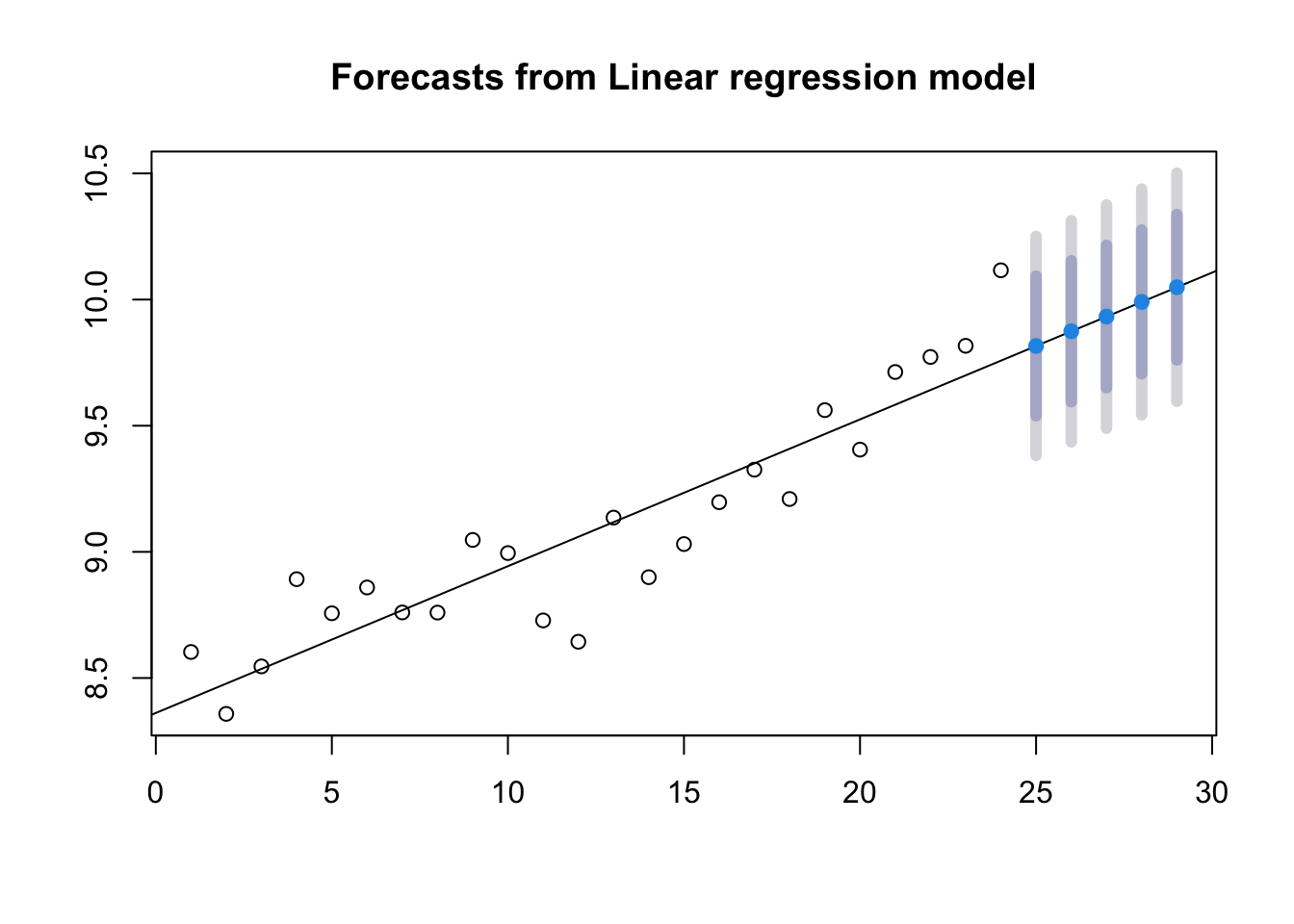
Anchovy forecasts from a higher order polynomial can similarly be made. Let’s fit a 4-th order polynomial.
\[C_t = \alpha + \beta_1 t + \beta_2 t^2 + \beta_3 t^3 + \beta_4 t^4 + e_t\]
To forecast with this model, we fit the model to estimate the \(\beta\)’s and then replace \(t\) with \(24\):
\[C_{1988} = \alpha + \beta_1 24 + \beta_2 24^2 + \beta_3 24^3 + \beta_4 24^4 + e_t\]
This is how to do that in R:
model <- lm(log.metric.tons ~ t + I(t^2) + I(t^3) + I(t^4), data=anchovy87)
fr <- forecast::forecast(model, newdata = data.frame(t=24:28))
fr
## Point Forecast Lo 80 Hi 80 Lo 95 Hi 95
## 1 10.05019 9.800941 10.29944 9.657275 10.44310
## 2 10.18017 9.856576 10.50377 9.670058 10.69028
## 3 10.30288 9.849849 10.75591 9.588723 11.01704
## 4 10.41391 9.770926 11.05689 9.400315 11.42750
## 5 10.50839 9.609866 11.40691 9.091963 11.92482Unfortunately, forecast’s plot() function for forecast objects does not recognize that there is only one predictor \(t\) thus we cannot use forecast’s plot function.
If you do this in R, it throws an error.
try(plot(fr))## Error in plotlmforecast(x, PI = PI, shaded = shaded, shadecols = shadecols, :
## Forecast plot for regression models only available for a single predictorError in plotlmforecast(x, PI = PI, shaded = shaded, shadecols = shadecols, : Forecast plot for regression models only available for a single predictorI created a function that you can use to plot time-varying regressions with polynomial \(t\). You will use this function in the lab.
plotforecasttv(model, ylims=c(8,17))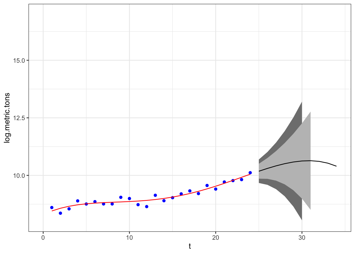
A feature of a time-varying regression with many polynomials is that it fits the data well, but the forecast quickly becomes uncertain due to uncertainty regarding the polynomial fit. A simpler model can give forecasts that do not become rapidly uncertain.
The flip-side is that the simpler model may not capture the short-term trends very well and may suffer from autocorrelated residuals.
model <- lm(log.metric.tons ~ t + I(t^2), data=anchovy87)plotforecasttv(model, ylims=c(8,17))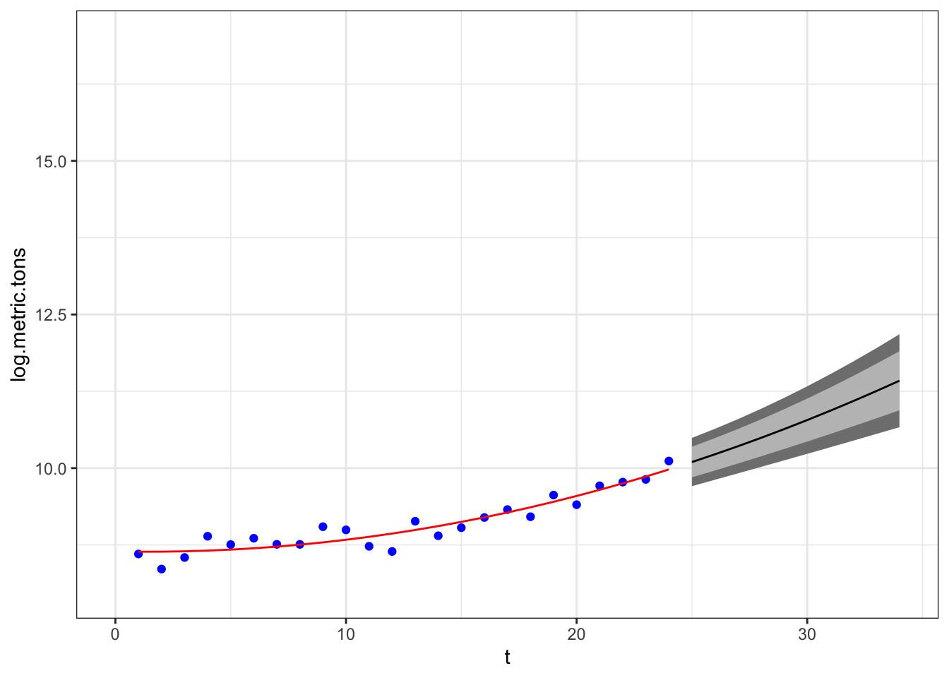
2.2.2 Summary
- Time-varying regression is a simple approach to forecasting that allows a non-linear trend.
- The uncertainty in your forecast is determined by how much error there is between the fit an the data.
- Fit must be balanced against prediction uncertainty.
- R allows you to quickly fit models and compute the prediction intervals.
Careful thought must be given to selecting the polynomial order.
- Standard methods are available in R for order selection
- Using different orders for different data sets has prediction consequences