4.2 Forecast performance

We can evaluate the forecast performance with forecasts of our test data or we can use all the data and use time-series cross-validation.

Let’s start with the former.

4.2.1 Test forecast performance

Test against a test data set

We will fit an an exponential smoothing model with trend to the training data and make a forecast for the years that we ‘held out’.

fit1 <- forecast::ets(traindat, model="AAN")
h=length(testdat)
fr <- forecast::forecast(fit1, h=h)
plot(fr)
points(testdat, pch=2, col="red")
legend("topleft", c("forecast","actual"), pch=c(20,2), col=c("blue","red"))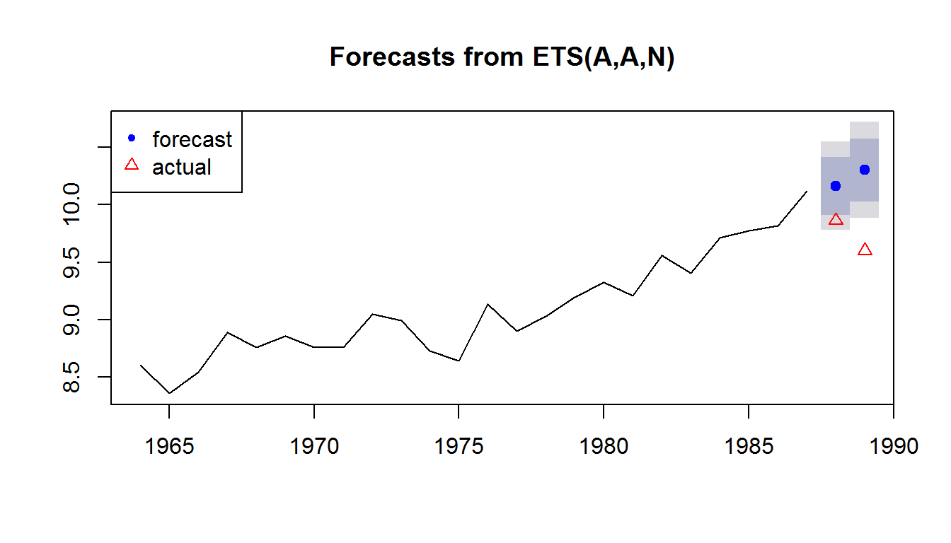

We can calculate a variety of forecast error metrics with

forecast::accuracy(fr, testdat)

##                      ME      RMSE       MAE        MPE     MAPE      MASE
## Training set  0.0155561 0.1788989 0.1442712  0.1272938 1.600532 0.7720807
## Test set     -0.5001701 0.5384355 0.5001701 -5.1678506 5.167851 2.6767060
##                      ACF1 Theil's U
## Training set -0.008371542        NA
## Test set     -0.500000000  2.690911

We would now repeat this for all the models in our candidate set and choose the model with the best forecast performance.

Test using time-series cross-validation

Another approach is to use all the data and test a series of forecasts made by fitting the model to different lengths of the data.

In this approach, we don’t have test data. Instead we will use all the data for fitting and for forecast testing.

We will redefine traindat as all our Anchovy data.

tsCV() function

We will use the tsCV() function. We need to define a function that returns a forecast.

far2 <- function(x, h, model){
  fit <- ets(x, model=model)
  forecast(fit, h=h)
  }

Now we can use tsCV() to run our far2() function to a series of training data sets. We will specify that a NEW ets model be estimated for each training set. We are not using the weighting estimated for the whole data set but estimating the weighting new for each set.

The e are our forecast errors for all the forecasts that we did with the data.

e <- forecast::tsCV(traindat, far2, h=1, model="AAN")
e

## Time Series:
## Start = 1964 
## End = 1989 
## Frequency = 1 
##  [1] -0.245378390  0.366852341  0.419678595 -0.414861770 -0.152727933
##  [6] -0.183775208 -0.013799590  0.308433377 -0.017680471 -0.329690537
## [11] -0.353441463  0.266143346 -0.110848616 -0.005227309  0.157821831
## [16]  0.196184446  0.008135667  0.326024067  0.085160559  0.312668447
## [21]  0.246437781  0.117274740  0.292601670 -0.300814605 -0.406118961
## [26]           NA

Let’s look at the first few e so we see exactly with tsCV() is doing.

e[2]

## [1] 0.3668523

This uses training data from \(t=1\) to \(t=2\) so fits an ets to the first two data points alone. Then it creates a forecast for \(t=3\) and compares that forecast to the actual value observed for \(t=3\).

TT <- 2 # end of the temp training data
temp <- traindat[1:TT]
fit.temp <- forecast::ets(temp, model="AAN")
fr.temp <- forecast::forecast(fit.temp, h=1)
traindat[TT+1] - fr.temp$mean

## Time Series:
## Start = 3 
## End = 3 
## Frequency = 1 
## [1] 0.3668523

e[3]

## [1] 0.4196786

TT <- 3 # end of the temp training data
temp <- traindat[1:TT]
fit.temp <- forecast::ets(temp, model="AAN")
fr.temp <- forecast::forecast(fit.temp, h=1)
traindat[TT+1] - fr.temp$mean

## Time Series:
## Start = 4 
## End = 4 
## Frequency = 1 
## [1] 0.4196786

Forecast accuracy metrics

Once we have the errors from tsCV(), we can compute forecast accuracy metrics.

RMSE: root mean squared error

rmse <- sqrt(mean(e^2, na.rm=TRUE))

MAE: mean absolute error

mae <- mean(abs(e), na.rm=TRUE)

4.2.2 Testing a specific ets model

By specifying model="AAN", we estimated a new ets model (meaning new weighting) for each training set used. We might want to specify that we use only the weighting we estimated for the full data set.

We do this by passing in a fit to model.

The e are our forecast errors for all the forecasts that we did with the data. fit1 below is the ets estimated from all the data 1964 to 1989. Note, the code will produce a warning that it is estimating the initial value and just using the weighting. That is what we want.

fit1 <- forecast::ets(traindat, model="AAN")
e <- forecast::tsCV(traindat, far2, h=1, model=fit1)
e

## Time Series:
## Start = 1964 
## End = 1989 
## Frequency = 1 
##  [1]           NA  0.576663901  1.031385937  0.897828249  1.033164616
##  [6]  0.935274283  0.958914499  1.265427119 -0.017241938 -0.332751184
## [11] -0.330473144  0.255886314 -0.103926617  0.031206730  0.154727479
## [16]  0.198328366 -0.020605522  0.297475742  0.005297401  0.264939892
## [21]  0.196256334  0.129798648  0.335887872 -0.074017535 -0.373267163
## [26]           NA